
This posting is an abbreviated version of a lecture given by Peter Sasieni at the Karolinska Institute on the occasion of the PhD thesis defence by Gabriel Isheden (His thesis is available to read here). The tradition at the Karolinska Institute is for the “opponent” to deliver a “popular science” talk in order to place the thesis in context. The thesis title is “Statistical models of breast cancer growth and spread”.
Who do you think you are?
The BBC have a series called “Who do you think you are?” in which a team of genealogists, archivists, and historians work with a celebrity to trace their ancestry. This lecture will take such an approach to trace the ancestry not of Gabriel, but of his thesis. Where do the ideas come from? Who were his intellectual ancestors? What great minds from European history have contributed to today’s PhD thesis.
Jeremy Bentham
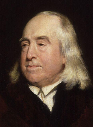
Jeremey Bentham (1748-1832) was the first to expound a utilitarian approach to society and ethics. He felt that the goal of society is to generate “the greatest good for the greatest number”. His work was the forerunner of cost-effectiveness analysis which is at the heart of health economic analysis which in turn provides a central motivation for the statistical modelling of tumour growth and spread.
The challenge of breast cancer screening that Gabriel Isheden seeks to address in his thesis is how best to allocate limited resources so as to have the greatest beneficial impact from breast screening without causing additional harm? It is impossible to do a large clinical trial of each and every permutation of breast cancer screening that one might propose, so inevitably we need to use modelling to ask the question: what do you think would happen if we were to screen like this?
Jeremy Bentham gave us a framework for looking at those model predictions and picking out what we think will be best for society.
Markov
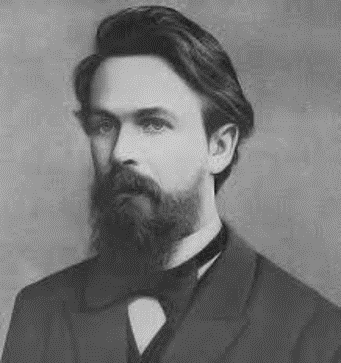
Andrey Markov (1856-1922) was one of those rare people whose name has become an adjective. Markov was a Russian mathematician who studied stochastic processes.
A stochastic process is simply a process describing the evolution over time of a random phenomenon. Stochastic processes have been used to describe the stock market, weather patterns, and, in today’s thesis, the spread of breast cancer to the lymph nodes.
In simple terms, a Markov process is one in which if you want to predict the future all you need to know is the present – there is no additional information to be gained from studying the past.
If you will excuse the cultural stereotyping, trains in Switzerland do not follow a Markov process but buses in England do. If in both countries there are three vehicles per hour, then in Switzerland knowing that someone has been waiting 14 minutes means that you would predict that on average then will need to wait another 3 minutes, whereas someone who has only been waiting 4 minutes will on average have to wait another 8 minutes; in England by contrast, we would predict a further 20 minute wait no long how long the person has already been waiting! This lack of memory is a Markov property.
Of course, buses in England do not run according to a Markov process – the time of one bus is not completely independent of the time of the previous bus, but I hope you get the idea.
Markov chains and disease progression
An early application of Markov chains to breast cancer modelling was from my long-term colleague and friend Stephen Duffy, working with his then boss, Nick Day, his now eminent PhD student Tony Chen and the distinguished Swedish radiologist Lazlo Tabar.
They proposed a simple three-state model in order to estimate how long breast cancer was potentially screen-detectable before being diagnosed without screening. Describing the distribution of the time spent in such a preclinical state is important for deciding how often women should be screened. They considered three states: no breast cancer; preclinical breast cancer; and clinical breast cancer. And assumed that there was no going back – once a woman had preclinical breast cancer, she would never return to the no breast cancer state without treatment.
Their model assumed that transitions between states were a bit like waiting for buses in England. But they didn’t assume that screening would always find breast cancer in a woman in the pre-clinical state. Rather they allowed for the screening test to have a certain probability of identifying cancer if it was there.
A few years later they considered a more complex model with five states. Noting that survival in women with breast cancer was much better if the cancer hadn’t spread to the lymph nodes and that some screen-detected cancer had already spread, they studied this model. Once again it was a Markov model.
Beyond five-state
But the three and even the five-state model is simplistic. Some would say overly simplistic. We know that tumours grow continuously and that the chance of detection on mammography increases the larger they are. For this reason, I think, Gabriel rejected the Markov model with a fixed sensitivity and instead uses a continuous growth model with a varying sensitivity.
Nevertheless, I hope he will agree that the mathematical approach to the study of stochastic process established by Markov was hugely important to his research.
Bayes
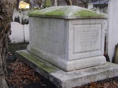
Next up is Thomas Bayes (1701-1761). He’s so old that we don’t have any pictures of him drawn before his death. So, he has been depicted here by his gravestone which is in Bunhill cemetery London, a short walk from Old Street roundabout.
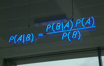
Bayes was a Presbyterian Minister and his eponymous theorem was only published posthumously. But it is so simple and so fundamental to probability theory and machine learning that it has been depicted in neon lights!
Bayes theorem is used multiple times in this thesis.
The model that Gabriel uses for growth is not really a stochastic process. Once we know the rate of growth of a given tumour, the growth is completely deterministic. But the rate of growth is random.
The idea of treating model parameters as random is often called Bayesian statistics, but there is little evidence that this is something that Thomas Bayes would have done!
Ada Lovelace
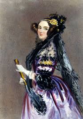
Ada Lovelace (1815-1852) also lived in England. She was the daughter of the poet Lord Byron but hardly knew him. She died young from cervical cancer, but despite my interest in that disease, it is not why she is in this lecture.
Ada Lovelace was a mathematician and is often credited as having written the first computer programme.
Without computer programmes Gabriel’s PhD thesis would not exist. So, her place in this ancestral hall of fame seems well justified.
Ludwig Boltzmann
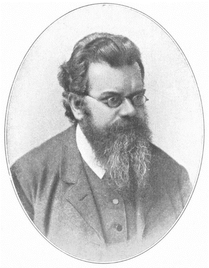
Ludwig Boltzmann (1844-1905) was an Austrian physicist. He is perhaps a strange choice for inclusion. He developed statistical mechanics and coined the term “ergodic”.
As this quote makes clear, he argued with James Clerk Maxwell (as in Maxwell’s equations of electromagnetism) on what one should mean by the probability of a state. (A state for us, might be having undiagnosed breast cancer). Boltzmann wanted to average over time for a given path, whereas Maxwell wanted to average over paths for a given time. When the two are equal, we say the process is ergodic.
Boltzmann, I think, also defined a stationary process as one whose distribution is time invariant.
As stationary ergodic process is one for which the average over time of a single curve is equal to the average of all curves at a given time.
Boltzmann made it into my compilation because reading Isheden’s Theorem 3, I was reminded of stationary ergodic processes. It seems to me that what Gabriel calls a stable process if very similar to a stationary process and his Theorem 3 is essentially stating that the growth process is ergodic.
Armitage & Doll
These two are the only ones of your distinguished ancestors who were alive when I was born. I am fortunate enough to have met them both. Peter Armitage a statistician is, as far as I know, still living in Oxford aged 95. Richard Doll was a physician and epidemiologist who inspired a whole generation of medical statisticians and epidemiologists. Best known for his work on tobacco, he died aged 92.
A paper of theirs from 1954 was a truly landmark contribution to the mathematical modelling of carcinogenesis which provided insights that also led to investigations in molecular biology. They observed that for many cancers the logarithm of mortality (as a surrogate for incidence) plotted against the logarithm of age formed a straight line with slope 5 or 6 and they postulated that this was in keeping with there being 6 or 7 ordered events necessary for cancer to occur.
Virchow
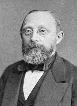
Rudolf Virchow (1821-1902) was a German physician who was made a foreign member of the Swedish Royal Academy of Sciences. He is often called the father of modern pathology. His contribution to this thesis is that he emphasized that disease arose primarily in individual cells.
He also did important early work on lymphatic drainage which is important for lymphatic spread studied by Gabriel.
Marie Curie
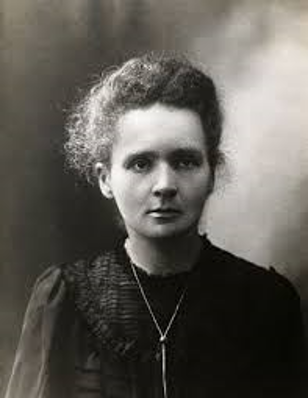
Marie Curie (1867-1934) could probably be credited with providing intellectual parentage to many PhD theses. She was the first person to win two Nobel prizes and is still the only person to win two in different scientific areas (one in physics and one in chemistry). Her many discoveries include important work on X ray imaging which is of course the basis for mammographic breast screening.
It might also be worth pointing out that she first won the Nobel prize in 1903 just six months after she was awarded her doctorate from the University of Paris. No pressure Gabriel!
This image is intended to help you understand why the sensitivity of breast screening is reduced in dense breasts. The four mammograms are from women with increasingly dense breasts.
The two hexagons in the rightmost black strip represent a small and a large breast cancer. Look at how they appear in the different breasts. Starting on the left, it is easy to spot even the small hexagon (I have not pasted the large one in the first two breasts). By the time we get to the third breast, you might struggle to see the small tumour, although the large one is not too difficult to locate.
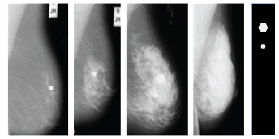
And in the fourth image, unless you are very good at looking at medical images, you probably can’t see the large hexagon.
Breast cancer survival
So why is all this important? Because even with modern treatments, the chance that a woman is alive 8 years after diagnosis with breast cancer depends critically on the size of the primary tumour and the spread to the axillary lymph nodes. Virtually no woman dies from a breast tumour that is less than 2.0cm in diameter, whereas over 20% of those with tumours over 5cm at diagnosis have died within 8 years. Similarly, virtually no one dies from a node-negative tumour, but nearly 40% of women in whom the cancer has spread to ten or more lymph nodes die within 8 years of diagnosis.
There is a lot of great research going on around the world by smart young students like Gabriel Isheden that is trying to address the question of how to better design cancer screening programmes so as to maximise the benefits and minimise the harms in an affordable way. That research rests on the intellectual contributions of geniuses from the 250 years.
The views expressed are those of the author. Posting of the blog does not signify that the Cancer Prevention Group endorse those views or opinions.
![]()